Microsoft Excelで検索機能を使用する方法

この記事では、MicrosoftExcelでSEARCH関数を使用する方法を学習します。

_MS-Excel SEARCH関数は、文字列内の部分文字列またはsearch_textの最初の文字の位置を返します。この関数は、検索中に大文字と小文字を区別しません。 FINDとは異なり、SEARCHでは疑問符（？）やアスタリスク（）などのワイルドカード文字を使用できます。疑問符（？）は任意の単一文字に一致し、アスタリスク（）は任意の文字シーケンスに一致します。

ただし、実際の疑問符（？）またはアスタリスク（*）を検索する場合は、文字の前に潮汐（〜）を入力します。部分文字列が文字列内に見つからない場合、関数は#VALUEエラーを返します。

SEARCH関数は、MID関数と組み合わせると強力な文字列メソッド関数として使用できます。_

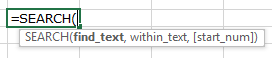
関数の引数/構文は次のとおりです：

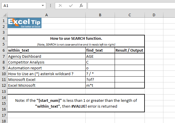
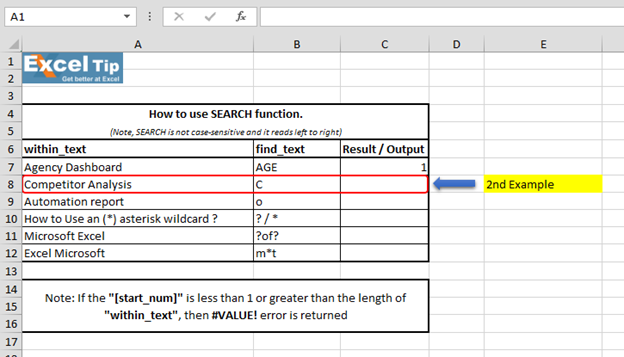
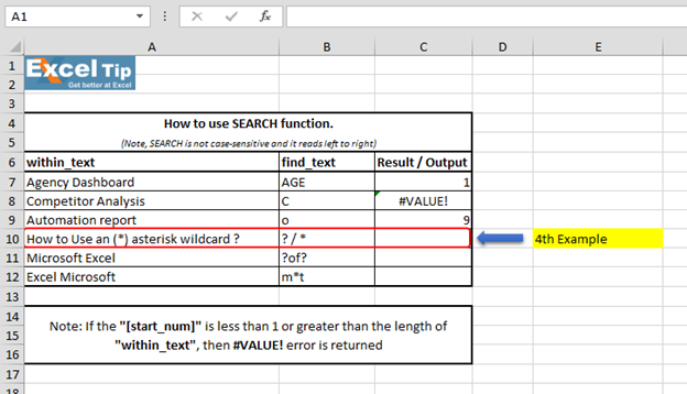
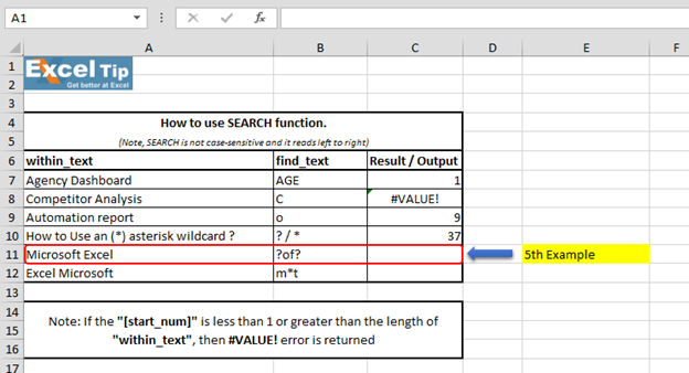
We have dummy data in column A. Column B contains the text which we will search for. And column C has the starting position of the search. And, here in column D, we will enter the SEARCH function.

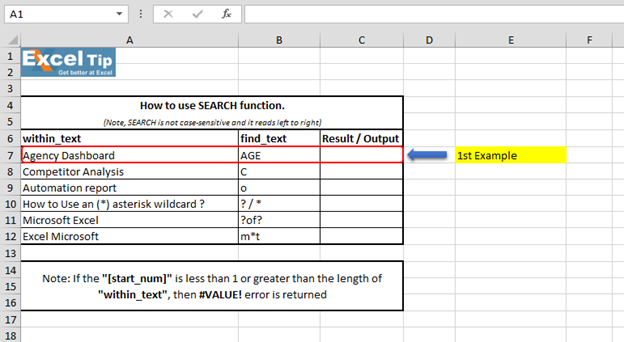
1^st Example:- In the first example, we will search “AGE” in cell A7.

Follow the steps given below:- Enter the function in cell C7 =SEARCH(“AGE”,A7,1)

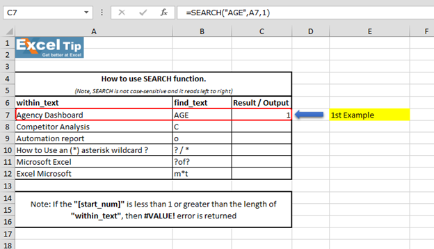It returns to 1 because “SEARCH” is looking from the first character, and it found AGE beginning from the 1^st character. So it gives us 1 here. 2^nd Example:- In this example, we will search for “C” and we give the starting number as zero or negative number as the starting position.

Follow the steps given below:- Enter the function in cell C8 =SEARCH(“c”,A8,-1), Press Enter

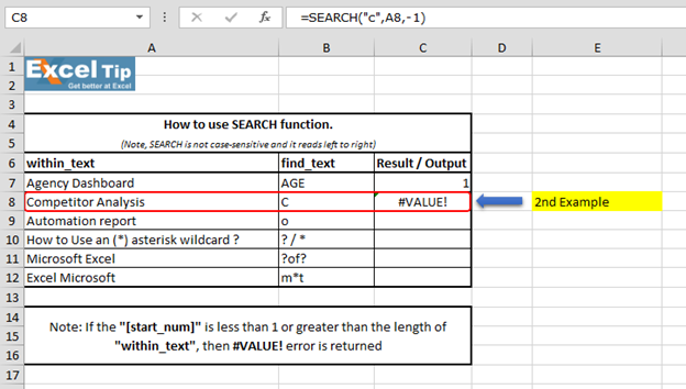The Function has returned #VALUE error because neither negative nor 0 can be the starting position. 3^rd Example:- In this example, we will show you what if we have to find the text which is there multiple times in the string.

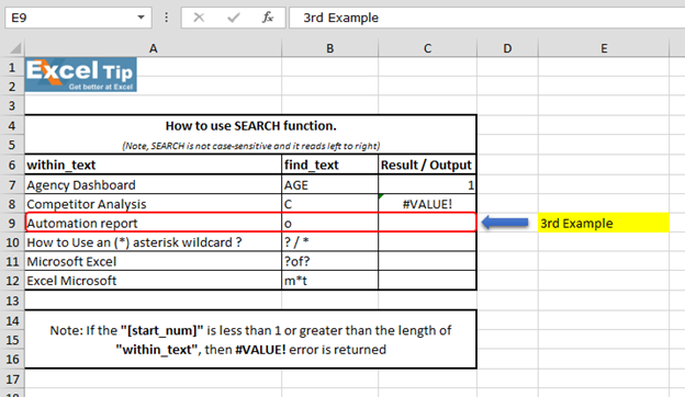Follow the steps given below:- Enter the function in cell C9 =SEARCH(“o”,A9,5), Press Enter

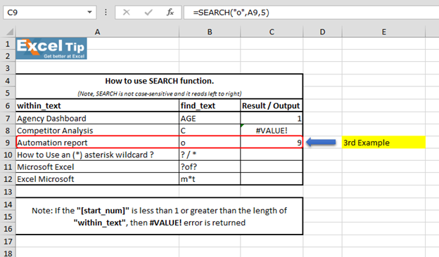The function has ignored the “o” which is at 4^th position and the function returns to 9 as the position. Because it ignored the first “o” and started looking from 5^th character onwards.

ただし、文字列の全体的な位置を返します。 4 ^ th ^例：-この例では、セルA10内のワイルドカード文字の位置を検索します。

Follow the steps given below:- First we’ll look for () asterisk sign, enter the function in cell C10 =SEARCH(“”,A10,1), Press Enter

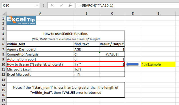The function has returned 1, because we cannot find any wildcard without using tilde. As we use tilde (~) as a marker to indicate that the next character is a literal, we will insert (~) tilde before (*) asterisk.

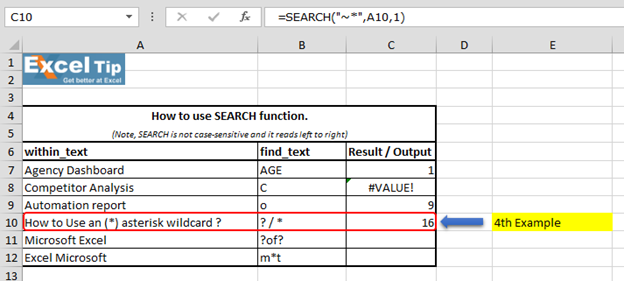
この関数を入力してください= SEARCH（ “〜”、A10,1）

We can also look for question mark:- Enter the function in same cell C10 =SEARCH(“~?”,A10,1), Press Enter

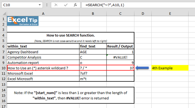We can see that function gave us “37” as the position of (?) question mark. 5^th Example:- In this example, we’ll learn how to enter SEARCH function to search “?of?”.

Follow the steps given below:- Enter the function in cell C11 =SEARCH(“?of?”,A11,1)

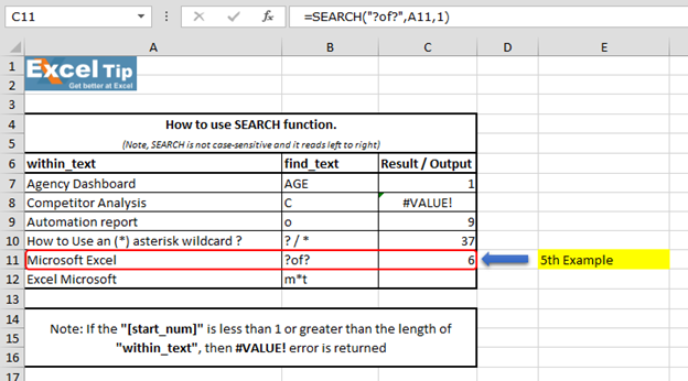We scan to see that function has returned 6 because it matches “soft” which is present in the mid of “Microsoft Excel” string and hence the value is 6. Note:- (?) question mark wildcard denotes any single character. 6^th Example:- In this example, we’ll learn another use of wildcard in SEARCH function.

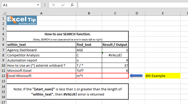Follow the steps given below:- Enter the function in cell C12 =SEARCH(“m*t”,A12,1)

注：-最初の引数では、「m」で始まり「t」で終わる文字列を検索するように関数に指示し、その間にアスタリスク（*）を置きます。

“Microsoft Excel” and it finds there is a string which starts with “M” and ends with “L”. No matter how many characters are there in between and hence it returns 1. Because (*)

アスタリスクのワイルド文字は、任意の文字シーケンスに一致します。つまり、これがさまざまな状況でSEARCH機能がどのように機能するかです。