Comment utiliser la fonction RECHERCHE dans Microsoft Excel

Dans cet article, nous allons apprendre à utiliser la fonction SEARCH dans Microsoft Excel.

_La fonction RECHERCHE MS-Excel renvoie la position du premier caractère de la sous-chaîne ou du texte de recherche dans une chaîne. La fonction ne fait pas de distinction entre les lettres majuscules et minuscules lors de la recherche. Contrairement à FIND, SEARCH autorise les caractères génériques, comme le point d’interrogation (?) Et l’astérisque (). Le point d’interrogation (?) Correspond à n’importe quel caractère et l’astérisque () correspond à n’importe quelle séquence de caractères.

Cependant, au cas où nous voudrions trouver un point d’interrogation (?) Ou un astérisque (*), nous tapons une marée (~) avant le caractère. Si la sous-chaîne n’est pas trouvée dans la chaîne, la fonction renverra l’erreur #VALUE.

La fonction SEARCH peut être utilisée comme une puissante fonction de méthode de chaîne lorsqu’elle est combinée avec la fonction MID._

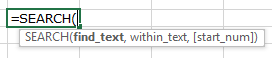
Les arguments / syntaxe de la fonction sont:

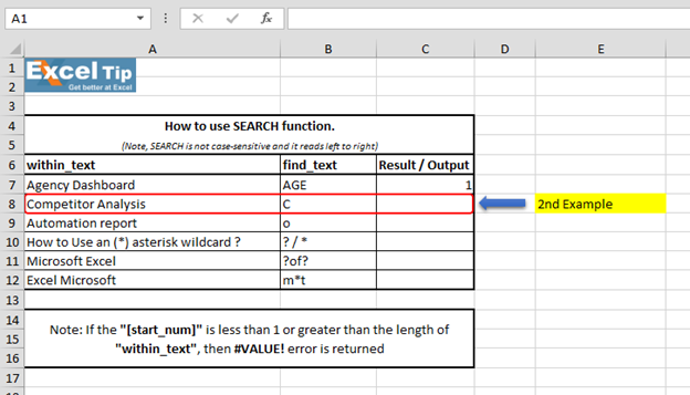
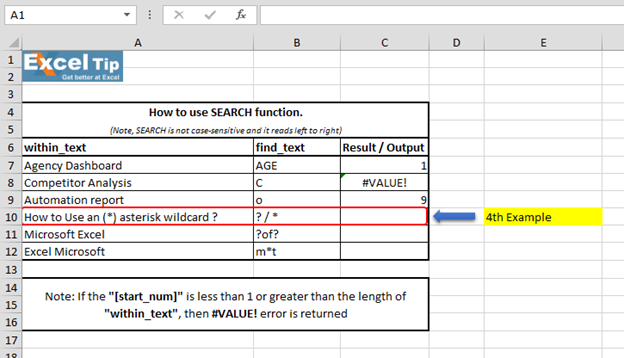
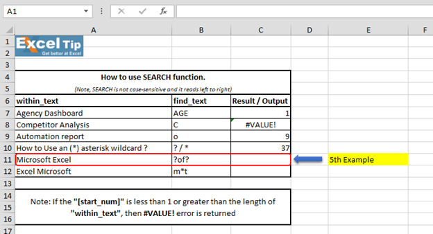
We have dummy data in column A. Column B contains the text which we will search for. And column C has the starting position of the search. And, here in column D, we will enter the SEARCH function.

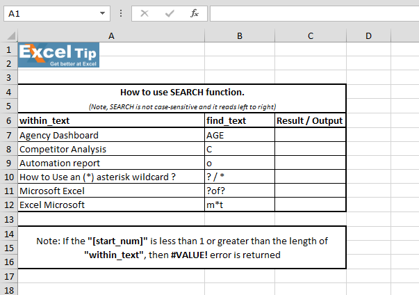1^st Example:- In the first example, we will search “AGE” in cell A7.

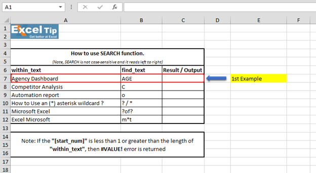Follow the steps given below:- Enter the function in cell C7 =SEARCH(« AGE »,A7,1)

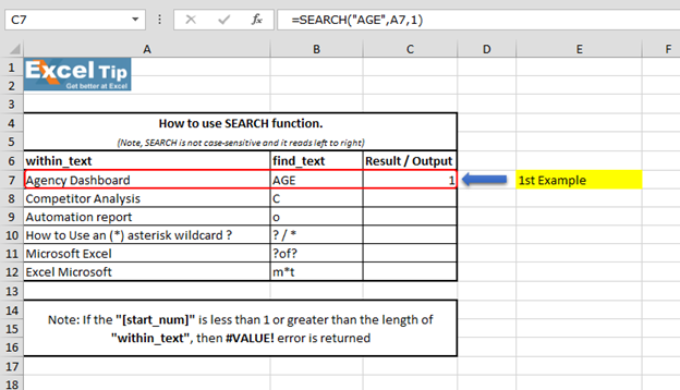It returns to 1 because “SEARCH” is looking from the first character, and it found AGE beginning from the 1^st character. So it gives us 1 here. 2^nd Example:- In this example, we will search for “C” and we give the starting number as zero or negative number as the starting position.

Follow the steps given below:- Enter the function in cell C8 =SEARCH(« c »,A8,-1), Press Enter

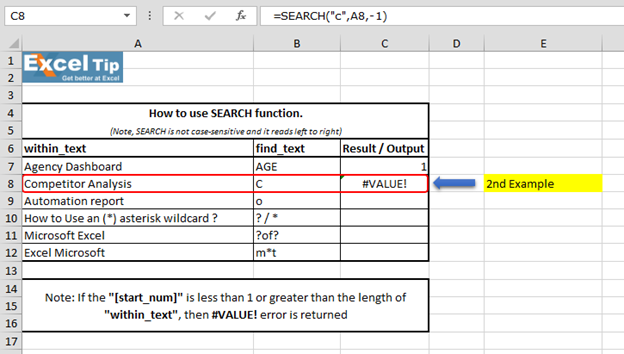The Function has returned #VALUE error because neither negative nor 0 can be the starting position. 3^rd Example:- In this example, we will show you what if we have to find the text which is there multiple times in the string.

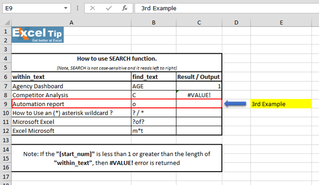Follow the steps given below:- Enter the function in cell C9 =SEARCH(« o »,A9,5), Press Enter

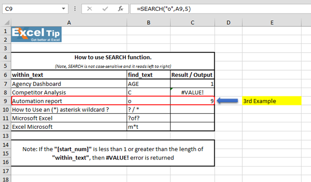The function has ignored the “o” which is at 4^th position and the function returns to 9 as the position. Because it ignored the first “o” and started looking from 5^th character onwards.

Cependant, il renvoie la position globale de la chaîne. 4 ^ th ^ Exemple: – Dans cet exemple, nous rechercherons la position des caractères génériques dans la cellule A10.

Follow the steps given below:- First we’ll look for () asterisk sign, enter the function in cell C10 =SEARCH(«  »,A10,1), Press Enter

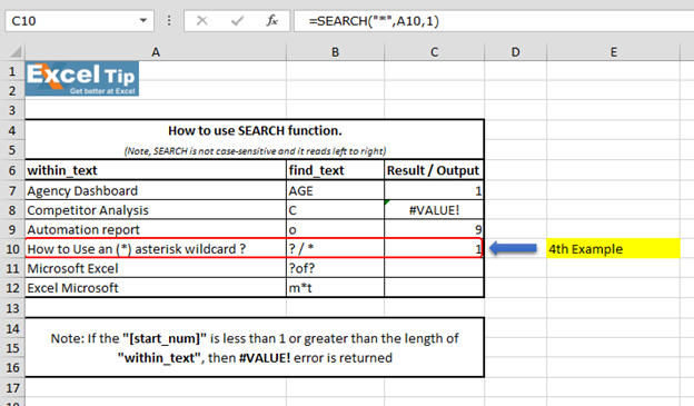The function has returned 1, because we cannot find any wildcard without using tilde. As we use tilde (~) as a marker to indicate that the next character is a literal, we will insert (~) tilde before (*) asterisk.

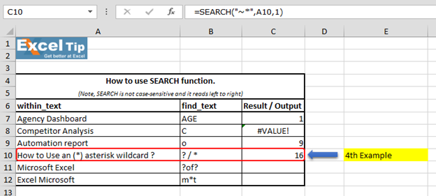
Entrez cette fonction = SEARCH (« ~ », A10,1)

We can also look for question mark:- Enter the function in same cell C10 =SEARCH(« ~? »,A10,1), Press Enter

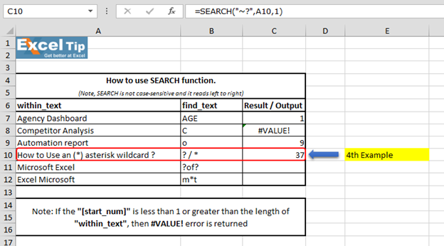We can see that function gave us “37” as the position of (?) question mark. 5^th Example:- In this example, we’ll learn how to enter SEARCH function to search “?of?”.

Follow the steps given below:- Enter the function in cell C11 =SEARCH(« ?of? »,A11,1)

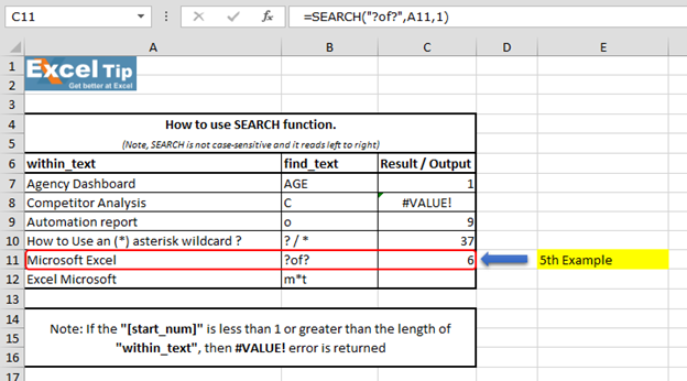We scan to see that function has returned 6 because it matches “soft” which is present in the mid of “Microsoft Excel” string and hence the value is 6. Note:- (?) question mark wildcard denotes any single character. 6^th Example:- In this example, we’ll learn another use of wildcard in SEARCH function.

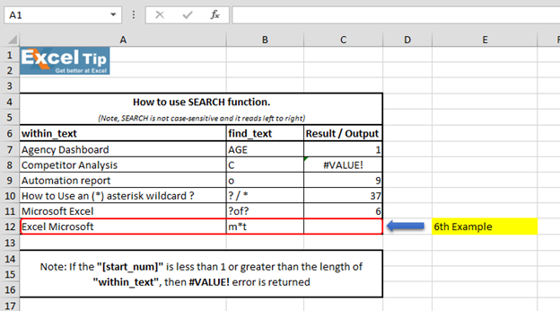Follow the steps given below:- Enter the function in cell C12 =SEARCH(« m*t »,A12,1)

Remarque: – Dans le premier argument, nous demandons à la fonction de rechercher la chaîne qui commence par «m» et se termine par «t», et nous mettrons un astérisque (*) entre les deux.

“Microsoft Excel” and it finds there is a string which starts with “M” and ends with “L”. No matter how many characters are there in between and hence it returns 1. Because (*)

Le caractère joker astérisque correspond à n’importe quelle séquence de caractères. Donc, voici comment la fonction de recherche fonctionne dans différentes situations.