How to Filter the Data in Excel using VBA

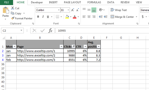
To understand how to put the filter, let’s take an example:- We have data in range A1:E35 in which column A contains Month, column B Page, column C Clicks, Column D CTR and column E contains average position.

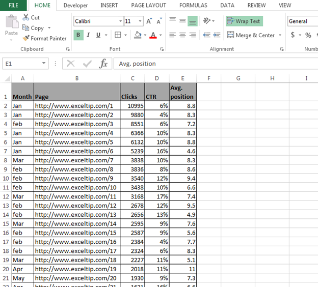
If we want to see the data of Jan month, then we need to put the filter on Jan month. To put the filter through VBA, follow below given steps:- * Open VBA Page press the key Alt+F11.

Sub Filterindata()

Range(“A1″).AutoFilter Field:=1, Criteria1:=”Jan”

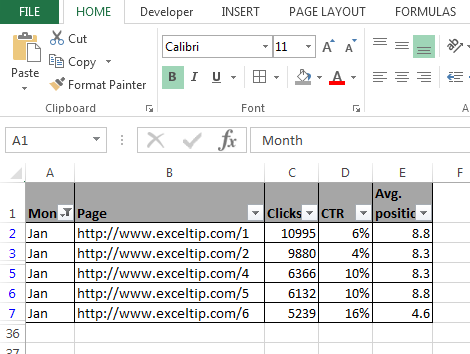
End Sub Code Explanation:- Firstly, we have to select the range of data where we want to put the filter and then we need to define the criteria.

To run the macro, press the key F5, and data will get filtered and we can see only Jan data.

To understand how to put the filter for bottom 10 items, let’s take an example:- We have data in range A1:E35 in which column A contains Month, column B Page, column C Clicks, Column D CTR and column E contains average position.

If we want to see the bottom 10 clicks in the data, then we need to follow below given steps:- * Open VBA Page press the key Alt+F11.

Sub filterbottom10()

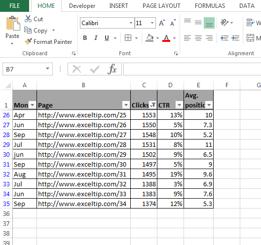
Range(“A1″).AutoFilter Field:=3, Criteria1:=”10”, Operator:=xlBottom10Items End Sub Code Explanation:- First, we have to select the range of data where we want to put the filter and then we need to define the criteria to filter the data of bottom 10 items.

To run the macro, press the key F5, and data will get filtered and we can see only bottom10 click’s data.

To understand how to put the filter for bottom 10 percent of data, let’s take an example:- We have data in range A1:E35 in which column A contains Month, column B Page, column C Clicks, Column D CTR and column E contains average position.

If we want to see the bottom 10 percent data, then we need to follow below given steps:- * Open VBA Page and press the key Alt+F11.

Sub Filterbottom10percent()

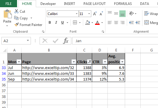
Range(“A1″).AutoFilter Field:=3, Criteria1:=”10”, Operator:=xlBottom10Percent End Sub Code Explanation:- First, we have to select the range of data where we want to put the filter and then we need to define the criteria to filter the data of bottom 10 percent.

To run the macro, press the key F5, and data will get filtered and we can see only bottom10 percent data.

To understand how to put the filter for bottom X numbers, let’s take an example:- We have data in range A1:E35 in which column A contains Month, column B Page, column C Clicks, Column D CTR and column E contains average position.

If we want to see the bottom x number of data, then we need to follow below given steps:- * Open VBA Page press the key Alt+F11.

Sub Filterbottomxnumber()

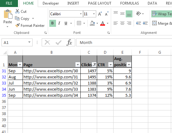
Range(“A1″).AutoFilter Field:=3, Criteria1:=”5”, Operator:=xlBottom10Items End Sub Code Explanation:- First we have select the range of data where we want to put the filter and then we gave the criteria to filter the 5 numbers of bottom 10 numbers.

To run the macro press the key F5, data will get filtered and we can see only bottom 10 click’s data.

To understand that how to put the filter for bottom x percent of data, let’s take an example:- We have data in range A1:E35, in which column A contains Month, column B Page, column C Clicks, Column D CTR and column E contains average position.

If we want to see the bottom x percent data, then we need to follow below given steps:- * Open VBA Page press the key Alt+F11.

Sub Filterbottomxpercent()

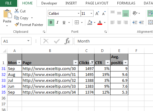
Range(“A1″).AutoFilter Field:=3, Criteria1:=”5”, Operator:=xlBottom10Percent End Sub Code Explanation:- First we have to select the range of data where we want to put the filter and then we need to define the criteria to filter the data of bottom x percent.

To run the macro, press the key F5, and data will get filtered and we can see only bottom 10 Percent data.

To understand how to put the filter for specific, let’s take an example:- We have data in range A1:E35 in which column A contains Month, column B Page, column C Clicks, Column D CTR and column E contains average position.

If we want to see the specific data only in column B, then we need to follow below given steps:- * Open VBA Page and press the key Alt+F11.

Sub Specificdata()

Range(“A1″).AutoFilter Field:=2, Criteria1:=”Exceltip”

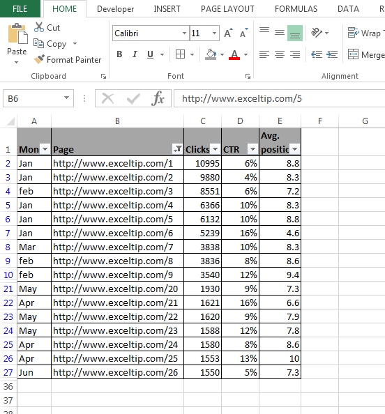
End Sub Code Explanation:- First we have select the range of data where we will define the column B in Field as 2 and then we will define that which data we want to see.

To run the macro press the key F5, data will get filtered and we can see only Exceltip’s data will appear.

To understand how to put the filter specifically, let’s take an example:- We have data in range A1:E35 in which column A contains Month, column B Page, column C Clicks, Column D CTR and column E contains average position.

If we want to see the data for Jan and Mar month, then we need to follow below given steps:- * Open VBA Page press the key Alt+F11.

Sub Multipledata()

Range(“A1:E1″).AutoFilter field:=1, Criteria1:=”Jan”, Operator:=xlAnd, Criteria2:=”Mar”

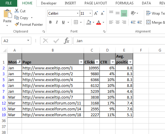
End Sub Code Explanation:- First we have to select the range of data where we will define the column A in Field as 1 and then we will define the both criteria.

To run the macro, press the key F5, and data will get filtered and we can see only Jan and Mar data will appear.

How to put the filter to display the records that contain a value between 2 values? To understand how to put the filter for multiple criteria, let’s take an example:- We have data in range A1:E35 in which column A contains Month, column B Page, column C Clicks, Column D CTR and column E contains average position.

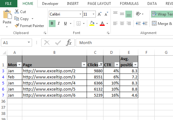
If we want to put the filter as per the criteria how many numbers we have under the clicks of 5000 to 10000 , follow below given steps:- * Open VBA Page and press the key Alt+F11.

Sub MultipleCriteria()

Range(“A1:E1″).AutoFilter field:=3, Criteria1:=”>5000″, Operator:=xlAnd, Criteria2:=”<10000″

End Sub Code Explanation: – First we have to select the range of data where we will define the criteria in column C by using operator function.

To run the macro, press the key F5, and data will get filtered and we can see the data as per the clicks which is more than 5000 and less than 10000.

To understand how to put the filter for multiple criteria in multiple columns, let’s take an example:- We have data in range A1:E35 in which column A contains Month, column B Page, column C Clicks, Column D CTR and column E contains average position.

Sub MultipleFields()

Range(“A1:E1″).AutoFilter field:=1, Criteria1:=”Jan”

Range(“A1:E1″).AutoFilter field:=2, Criteria1:=”Exceltip”

End Sub Code Explanation: – Firstly, we have to select the range of data where we want to put the filter and then we will have to define the criteria 2 times to achieve the target.

To understand how to filter the data without applying the filter in column, let’s take an example:- We have data in range A1:E35 in which column A contains Month, column B Page, column C Clicks, Column D CTR and column E contains average position.

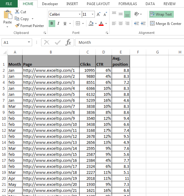
If we want to put the filter for in Jan month and hide the filter arrow in the field, follow below given steps:- * Open VBA Page press the key Alt+F11.

Sub HideFilter()

Range(“A1″).AutoFilter field:=1, Criteria1:=”Jan”, visibledropdown:=False End Sub Code Explanation: – First, we have to select the range of data where we want to put the filter and then we need to make sure that filter should not be visible.

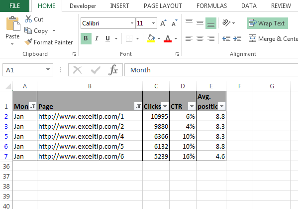
To run the macro, press the key F5, and data will get filtered. Now, we can see the data in Jan month’s data only but the filter arrow will not appear in month’s column.

To understand how to filter the data to display the 1 or 2 possible values, let’s take an example:- We have data in range A1:E35 in which column A contains Month, column B Page, column C Clicks, Column D CTR and column E contains average position.

If we want to put the filter in Jan month and hide the filter arrow in the field, we need to follow below given steps:- * Open VBA Page press the key Alt+F11.

Sub HideFilter()

Range(“A1″).AutoFilter field:=1, Criteria1:=”Jan”, visibledropdown:=False End Sub Code Explanation: – Firstly, we have to select the range of data where we want to put the filter and then we will make sure that filter should not be visible.

To run the macro, press the key F5, and data will get filtered. Now, we can see the data in Jan month’s data and Feb month’s data.

To understand how to put the filter for top 10 items, let’s take an example:- We have data in range A1:E35 in which column A contains Month, column B Page, column C Clicks, Column D CTR and column E contains average position.

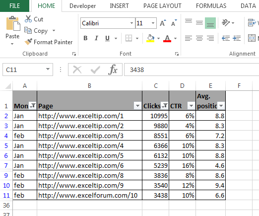
If we want to see the top 10 clicks in the data, then we need to follow below given steps:- * Open VBA Page and press the key Alt+F11.

Sub filtertop10()

Range(“A1″).AutoFilter Field:=3, Criteria1:=”10”, Operator:=xlTop10Items End Sub Code Explanation- Firstly, we have to select the range of data where we want to put the filter and then we need to define the criteria to filter the data from top 10 items.

To run the macro, press the key F5, and data will get filtered and we can see only top 10 click’s data.

To understand how to put the filter for top 10 percent of data, let’s take an example:- We have data in range A1:E35 in which column A contains Month, column B Page, column C Clicks, Column D CTR and column E contains average position.

If we want to see the top 10 percent data, then we need to follow below given steps:- * Open VBA Page press the key Alt+F11.

Sub Filtertop10percent()

Range(“A1″).AutoFilter Field:=3, Criteria1:=”10”, Operator:=xlTop10Percent End Sub Code Explanation:- First we have to select the range of data where we want to put the filter and then we need to define the criteria to filter the data from top 10 percent.

To run the macro, press the key F5, and data will get filtered. Now, we can see only top 10 percent data.

To understand how to remove the filter, follow below given steps:- * Open VBA Page press the key Alt+F11.

Sub removefilter()

Worksheets(“Sheet1”).ShowAllData End Sub To run the macro press the key F5, all data will get show but filter arrow will not be remove.

This is all about how we can put the filters through VBA in Microsoft Excel.