如何使用搜索功能在Microsoft Excel

在本文中，我们将学习如何在Microsoft Excel中使用SEARCH函数。

_MS-Excel SEARCH函数返回字符串中子字符串或search_text的第一个字符的位置。搜索时，该功能不会区分大小写字母。与FIND不同，SEARCH允许使用通配符，例如问号（？）和星号（）。问号（？）匹配任何单个字符，星号（）匹配任何字符序列。

但是，如果要查找实际的问号（？）或星号（*），请在字符前面键入一个潮汐（〜）。如果在字符串中未找到子字符串，则该函数将返回#VALUE错误。

与MID函数结合使用时，SEARCH函数可以用作强大的字符串方法函数。_

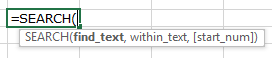
函数参数/语法为：

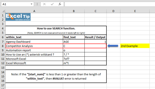
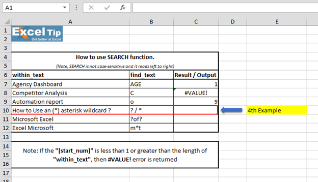
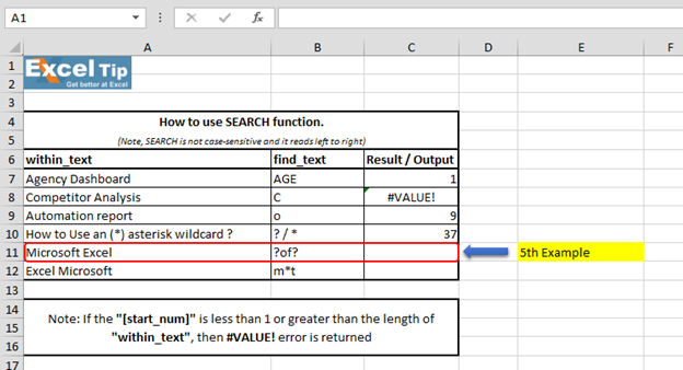
We have dummy data in column A. Column B contains the text which we will search for. And column C has the starting position of the search. And, here in column D, we will enter the SEARCH function.

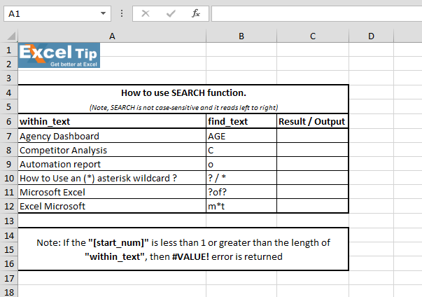1^st Example:- In the first example, we will search “AGE” in cell A7.

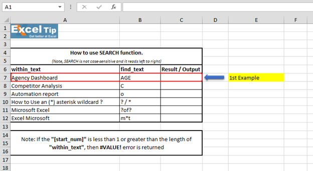Follow the steps given below:- Enter the function in cell C7 =SEARCH(“AGE”,A7,1)

It returns to 1 because “SEARCH” is looking from the first character, and it found AGE beginning from the 1^st character. So it gives us 1 here. 2^nd Example:- In this example, we will search for “C” and we give the starting number as zero or negative number as the starting position.

Follow the steps given below:- Enter the function in cell C8 =SEARCH(“c”,A8,-1), Press Enter

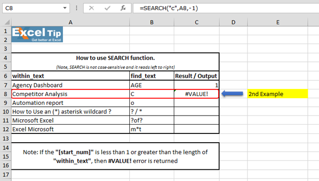The Function has returned #VALUE error because neither negative nor 0 can be the starting position. 3^rd Example:- In this example, we will show you what if we have to find the text which is there multiple times in the string.

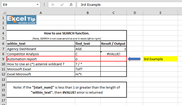Follow the steps given below:- Enter the function in cell C9 =SEARCH(“o”,A9,5), Press Enter

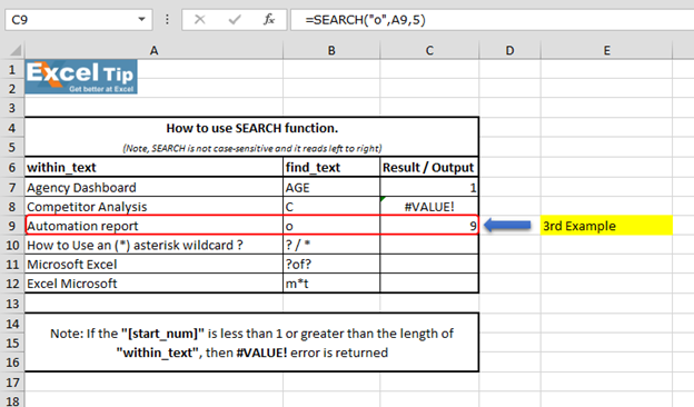The function has ignored the “o” which is at 4^th position and the function returns to 9 as the position. Because it ignored the first “o” and started looking from 5^th character onwards.

但是，它返回字符串的整体位置。第4 ^ th ^示例：-在此示例中，我们将在单元格A10中搜索通配符的位置。

Follow the steps given below:- First we’ll look for () asterisk sign, enter the function in cell C10 =SEARCH(“”,A10,1), Press Enter

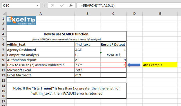The function has returned 1, because we cannot find any wildcard without using tilde. As we use tilde (~) as a marker to indicate that the next character is a literal, we will insert (~) tilde before (*) asterisk.

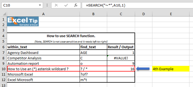
输入此函数= SEARCH（“〜”，A10,1）

We can also look for question mark:- Enter the function in same cell C10 =SEARCH(“~?”,A10,1), Press Enter

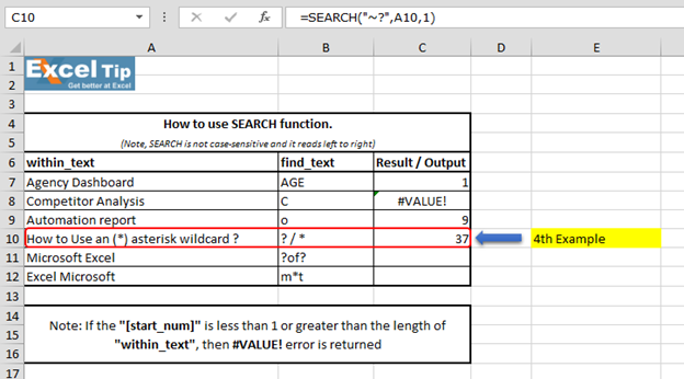We can see that function gave us “37” as the position of (?) question mark. 5^th Example:- In this example, we’ll learn how to enter SEARCH function to search “?of?”.

Follow the steps given below:- Enter the function in cell C11 =SEARCH(“?of?”,A11,1)

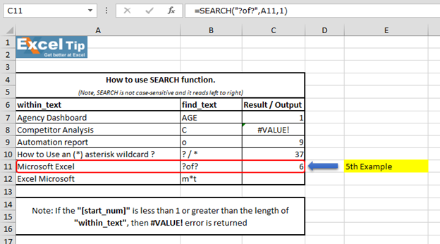We scan to see that function has returned 6 because it matches “soft” which is present in the mid of “Microsoft Excel” string and hence the value is 6. Note:- (?) question mark wildcard denotes any single character. 6^th Example:- In this example, we’ll learn another use of wildcard in SEARCH function.

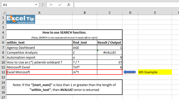Follow the steps given below:- Enter the function in cell C12 =SEARCH(“m*t”,A12,1)

注意：-在第一个参数中，我们告诉函数查找以“ m”开头和以“ t”结尾的字符串，并在它们之间插入星号（*）。

“Microsoft Excel” and it finds there is a string which starts with “M” and ends with “L”. No matter how many characters are there in between and hence it returns 1. Because (*)

星号百搭字符匹配任何字符序列。因此，这就是SEARCH功能在不同情况下的工作方式。