Come utilizzare la funzione di ricerca di Microsoft Excel

_ In questo articolo impareremo come usare la funzione RICERCA in Microsoft Excel._

_La funzione RICERCA MS-Excel restituisce la posizione del primo carattere della sottostringa o del testo_ricerca in una stringa. La funzione non distingue tra lettere maiuscole e minuscole durante la ricerca. A differenza di TROVA, RICERCA consente caratteri jolly, come il punto interrogativo (?) E l’asterisco (). Il punto interrogativo (?) Corrisponde a qualsiasi carattere singolo e l’asterisco () corrisponde a qualsiasi sequenza di caratteri.

Tuttavia, nel caso in cui desideriamo trovare un vero punto interrogativo (?) O un asterisco (*), digitiamo una marea (~) prima del carattere. Se la sottostringa non viene trovata all’interno della stringa, la funzione restituirà l’errore #VALUE.

La funzione SEARCH può essere utilizzata come potente funzione di metodo stringa se combinata con la funzione MID ._

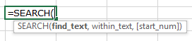
Gli argomenti / sintassi della funzione sono:

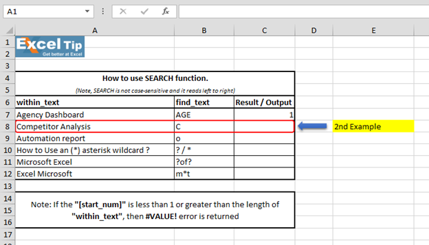
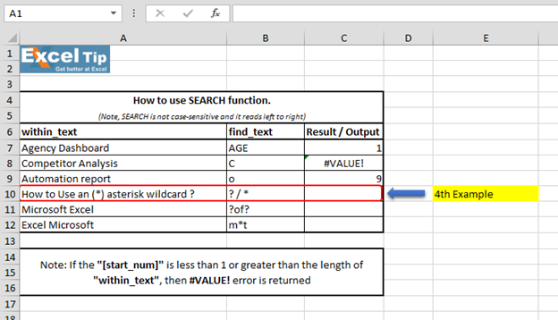
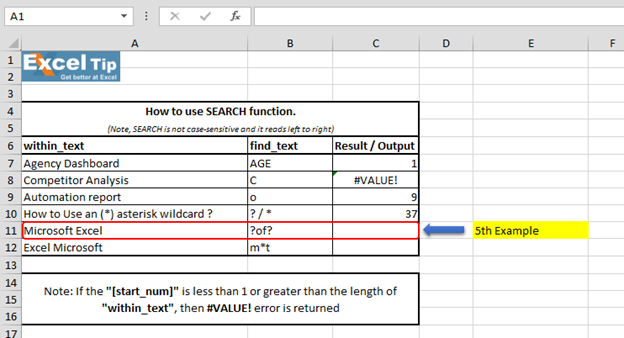
We have dummy data in column A. Column B contains the text which we will search for. And column C has the starting position of the search. And, here in column D, we will enter the SEARCH function.

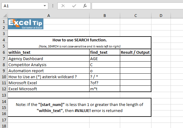1^st Example:- In the first example, we will search “AGE” in cell A7.

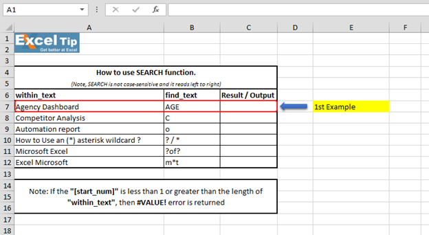Follow the steps given below:- Enter the function in cell C7 =SEARCH(“AGE”,A7,1)

It returns to 1 because “SEARCH” is looking from the first character, and it found AGE beginning from the 1^st character. So it gives us 1 here. 2^nd Example:- In this example, we will search for “C” and we give the starting number as zero or negative number as the starting position.

Follow the steps given below:- Enter the function in cell C8 =SEARCH(“c”,A8,-1), Press Enter

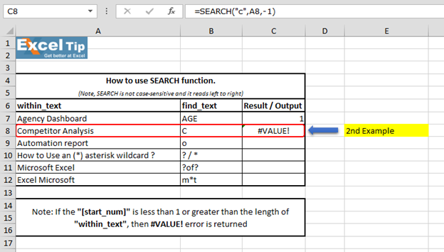The Function has returned #VALUE error because neither negative nor 0 can be the starting position. 3^rd Example:- In this example, we will show you what if we have to find the text which is there multiple times in the string.

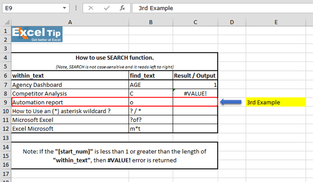Follow the steps given below:- Enter the function in cell C9 =SEARCH(“o”,A9,5), Press Enter

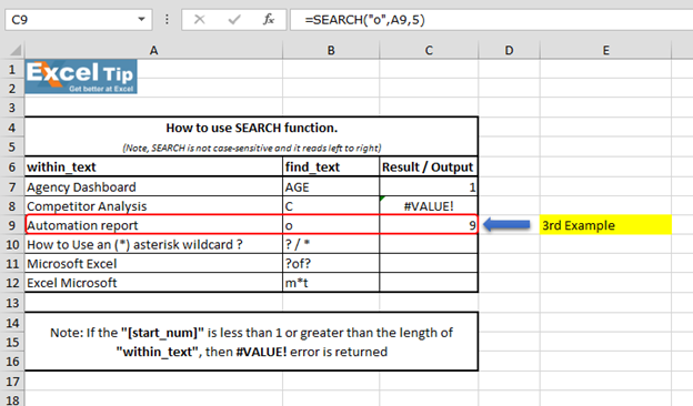The function has ignored the “o” which is at 4^th position and the function returns to 9 as the position. Because it ignored the first “o” and started looking from 5^th character onwards.

Tuttavia, restituisce la posizione complessiva della stringa. 4 ^ ^ Esempio: – In questo esempio, cercheremo la posizione dei caratteri jolly all’interno della cella A10.

Follow the steps given below:- First we’ll look for () asterisk sign, enter the function in cell C10 =SEARCH(“”,A10,1), Press Enter

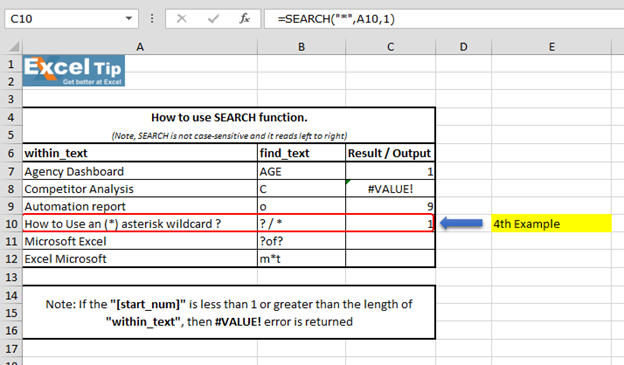The function has returned 1, because we cannot find any wildcard without using tilde. As we use tilde (~) as a marker to indicate that the next character is a literal, we will insert (~) tilde before (*) asterisk.

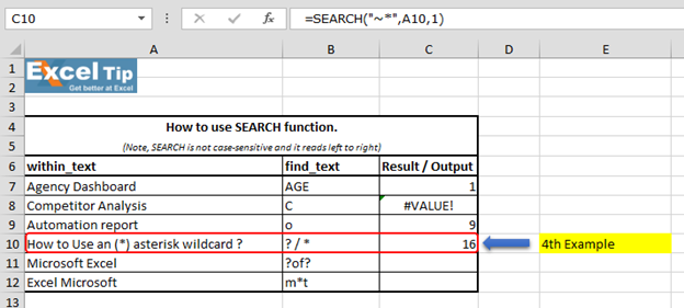
Immettere questa funzione = SEARCH (“~”, A10,1)

We can also look for question mark:- Enter the function in same cell C10 =SEARCH(“~?”,A10,1), Press Enter

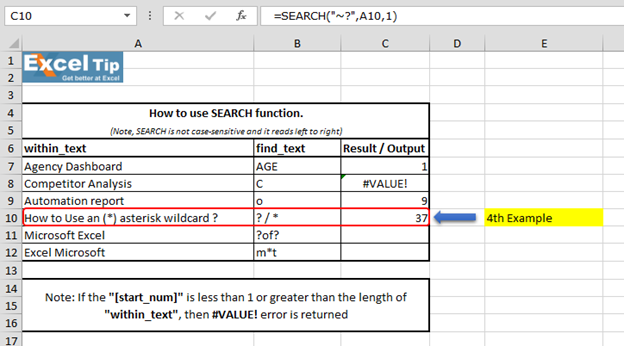We can see that function gave us “37” as the position of (?) question mark. 5^th Example:- In this example, we’ll learn how to enter SEARCH function to search “?of?”.

Follow the steps given below:- Enter the function in cell C11 =SEARCH(“?of?”,A11,1)

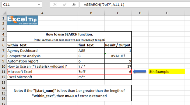We scan to see that function has returned 6 because it matches “soft” which is present in the mid of “Microsoft Excel” string and hence the value is 6. Note:- (?) question mark wildcard denotes any single character. 6^th Example:- In this example, we’ll learn another use of wildcard in SEARCH function.

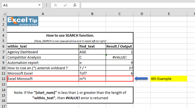Follow the steps given below:- Enter the function in cell C12 =SEARCH(“m*t”,A12,1)

Nota: – Nel primo argomento, diciamo alla funzione di cercare la stringa che inizia con “m” e finisce con “t”, inserendo l’asterisco (*) in mezzo.

“Microsoft Excel” and it finds there is a string which starts with “M” and ends with “L”. No matter how many characters are there in between and hence it returns 1. Because (*)

il carattere jolly asterisco corrisponde a qualsiasi sequenza di caratteri. Quindi, questo è il modo in cui funziona la funzione RICERCA in situazioni diverse.