엑셀 천장 기능
이 기사에서는 Excel에서 CEILING 함수를 사용하는 방법에 대해 알아 봅니다.
CEILING 함수는 Excel의 Math 또는 Trig 함수가 여러 중요도를 기준으로 반올림 된 숫자를 반환하는 범주입니다.
간단히 말해서 Excel CEILING 함수는 Excel의`link : / mathematical-functions-excel-mround-function [MROUND function]`처럼 작동합니다. 이 함수는 항상 유효 숫자로 반올림됩니다
구문
=CEILING (number, Significance)
숫자 : 반올림 할 숫자입니다.
의미 : 숫자로 반올림됩니다.
아래 표시된 데이터 범위에서이 기능을 사용해 보겠습니다.
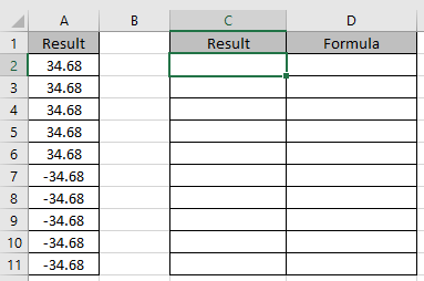
여기에 5 개의 양의 값과 5 개의 음의 값이 있습니다. 우리는 다른 유효 숫자를 사용할 것입니다.
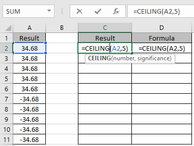
공식 사용 :
=CEILING(A2, 5)
Ctrl D
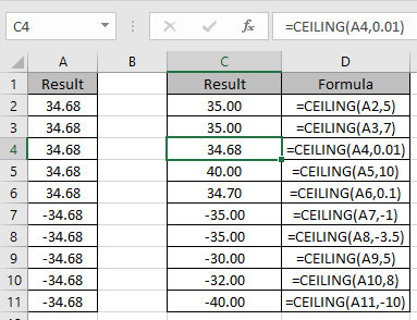
를 사용하여 전체 출력을 얻으려면 나머지 셀에 수식을 복사하십시오. 보시다시피 유의 수가 항상 다양하기 때문에 출력으로 다른 수를 얻었습니다.
CEILING 함수를 사용하여 Excel에서 숫자를 반올림하는 방법을 이해 하셨기를 바랍니다. 여기에서 Excel 기능에 대한 더 많은 기사를 살펴보십시오. 위의 기사에 대한 질문이나 피드백을 자유롭게 말씀해주십시오.
관련 기사 :
link : / statistical-formulas-how-to-use-the-floor-math-function-in-excel [Excel에서 FLOOR.MATH 함수 사용 방법]
link : / excel-format-using-the-round-function-to-round-numbers-to-thousands [수식 반올림 : 가장 가까운 100과 1000]
link : / mathematical-functions-excel-round-function [Excel에서 Round 함수를 사용하는 방법]
link : / mathematical-functions-excel-roundup-function [Excel에서 RoundUp 함수 사용 방법]
link : / mathematical-functions-excel-rounddown-function [Excel에서 반올림 함수 사용 방법]
link : / other-qa-formulas-rounding-numerical-calculation-results-in-microsoft-excel [Microsoft Excel의 반올림 수치 계산 결과]
인기 기사 :
link : / keyboard-formula-shortcuts-50-excel-shortcuts-to-increase-your-productivity [50 Excel 단축키로 생산성 향상]
link : / formulas-and-functions-introduction-of-vlookup-function [Excel에서 VLOOKUP 함수를 사용하는 방법]
link : / tips-countif-in-microsoft-excel [Excel 2016에서 COUNTIF 함수를 사용하는 방법]
link : / excel-formula-and-function-excel-sumif-function [Excel에서 SUMIF 함수 사용 방법]