어떻게 Microsoft Excel에서 검색 기능을 사용하는

이 기사에서는 Microsoft Excel에서 SEARCH 기능을 사용하는 방법을 배웁니다 .

_MS-Excel SEARCH 함수는 문자열에서 하위 문자열 또는 search_text의 첫 번째 문자의 위치를 ​​반환합니다. 이 기능은 검색하는 동안 대문자와 소문자를 구별하지 않습니다. FIND와 달리 SEARCH는 물음표 (?) 및 별표 ()와 같은 와일드 카드 문자를 허용합니다. 물음표 (?)는 단일 문자와 일치하고 별표 ()는 모든 문자 시퀀스와 일치합니다.

그러나 실제 물음표 (?) 또는 별표 (*)를 찾으려면 문자 앞에 조수 (~)를 입력합니다. 문자열 내에서 하위 문자열을 찾을 수없는 경우 함수는 #VALUE 오류를 반환합니다.

SEARCH 기능은 MID 기능과 결합하면 강력한 문자열 메소드 기능으로 사용할 수 있습니다 ._

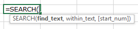
함수 인수 / 구문은 다음과 같습니다.

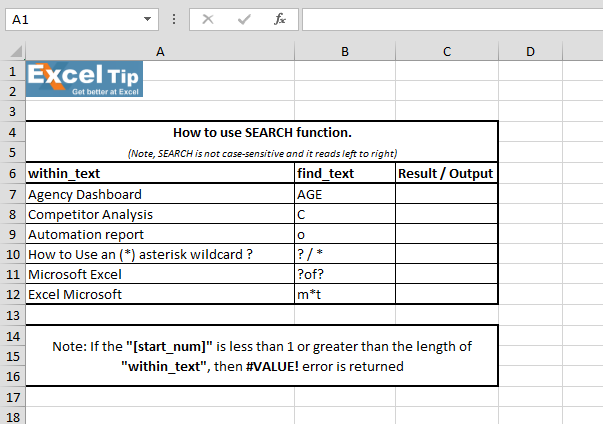
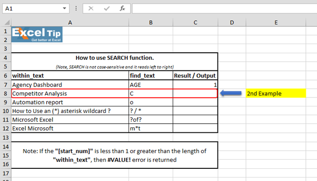
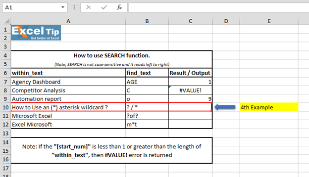
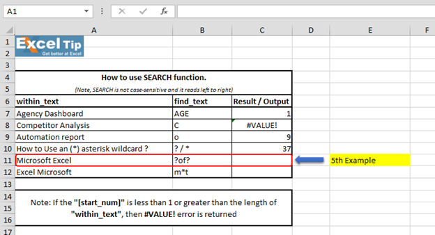
We have dummy data in column A. Column B contains the text which we will search for. And column C has the starting position of the search. And, here in column D, we will enter the SEARCH function.

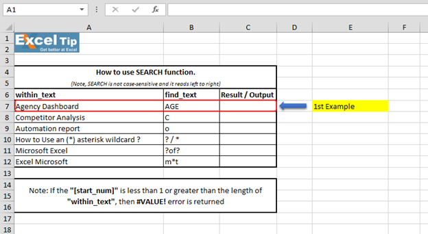
1^st Example:- In the first example, we will search “AGE” in cell A7.

Follow the steps given below:- Enter the function in cell C7 =SEARCH(“AGE”,A7,1)

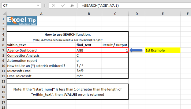It returns to 1 because “SEARCH” is looking from the first character, and it found AGE beginning from the 1^st character. So it gives us 1 here. 2^nd Example:- In this example, we will search for “C” and we give the starting number as zero or negative number as the starting position.

Follow the steps given below:- Enter the function in cell C8 =SEARCH(“c”,A8,-1), Press Enter

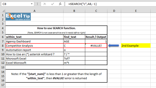The Function has returned #VALUE error because neither negative nor 0 can be the starting position. 3^rd Example:- In this example, we will show you what if we have to find the text which is there multiple times in the string.

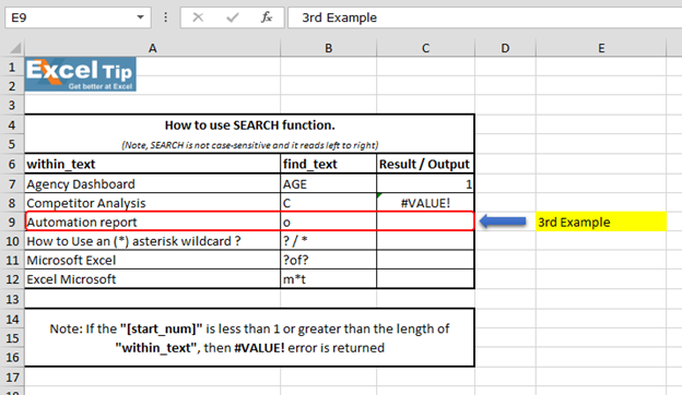Follow the steps given below:- Enter the function in cell C9 =SEARCH(“o”,A9,5), Press Enter

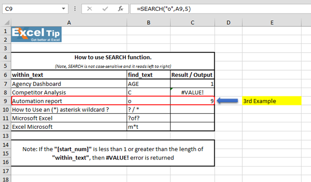The function has ignored the “o” which is at 4^th position and the function returns to 9 as the position. Because it ignored the first “o” and started looking from 5^th character onwards.

그러나 문자열의 전체 위치를 반환합니다. 4 ^ th ^ 예 :-이 예에서는 A10 셀 내에서 와일드 카드 문자의 위치를 ​​검색합니다.

Follow the steps given below:- First we’ll look for () asterisk sign, enter the function in cell C10 =SEARCH(“”,A10,1), Press Enter

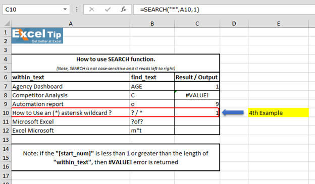The function has returned 1, because we cannot find any wildcard without using tilde. As we use tilde (~) as a marker to indicate that the next character is a literal, we will insert (~) tilde before (*) asterisk.

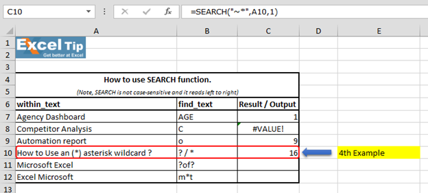
이 함수 입력 = SEARCH ( “~”, A10,1)

We can also look for question mark:- Enter the function in same cell C10 =SEARCH(“~?”,A10,1), Press Enter

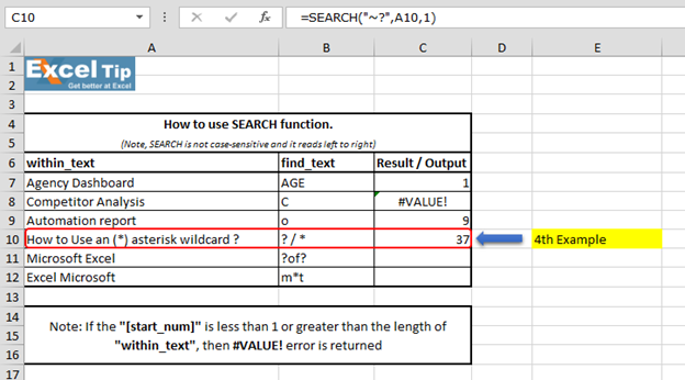We can see that function gave us “37” as the position of (?) question mark. 5^th Example:- In this example, we’ll learn how to enter SEARCH function to search “?of?”.

Follow the steps given below:- Enter the function in cell C11 =SEARCH(“?of?”,A11,1)

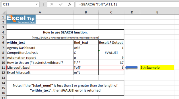We scan to see that function has returned 6 because it matches “soft” which is present in the mid of “Microsoft Excel” string and hence the value is 6. Note:- (?) question mark wildcard denotes any single character. 6^th Example:- In this example, we’ll learn another use of wildcard in SEARCH function.

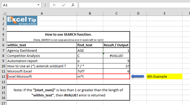Follow the steps given below:- Enter the function in cell C12 =SEARCH(“m*t”,A12,1)

참고 :-첫 번째 인수에서 “m”으로 시작하고 “t”로 끝나는 문자열을 찾도록 함수에 지시하고 그 사이에 별표 (*)를 넣습니다.

“Microsoft Excel” and it finds there is a string which starts with “M” and ends with “L”. No matter how many characters are there in between and hence it returns 1. Because (*)

별표 와일드 문자는 모든 문자 시퀀스와 일치합니다. 그래서 이것이 다른 상황에서 SEARCH 기능이 작동하는 방식입니다.